This notebook presents a rather complete overview of the syntax of Euler Math Toolbox (EMT), including its numerical and symbolic commands, variables and assignments.
We start with command lines.
An Euler command can be an expression or a primitive command. An expression is made of operators and functions. If necessary, it must contain brackets to force the correct order of execution. In doubt, setting a bracket is a good idea. Note that EMT shows opening and closing brackets while editing the command line.
>(cos(pi/4)+1)^3*(sin(pi/4)+1)^2
14.4978445072
The numerical operators of Euler include
 + unary or operator plus
 - unary or operator minus
 *, /
 . the matrix product
 a^b power for positive a or integer b (a**b works too)
 n! the factorial operator
and many more.
Here are some of the functions you might need. There are many more.
 sin,cos,tan,atan,asin,acos,rad,deg
 log,exp,log10,sqrt,logbase
 bin,logbin,logfac,mod,floor,ceil,round,abs,sign
 conj,re,im,arg,conj,real,complex
 beta,betai,gamma,complexgamma,ellrf,ellf,ellrd,elle
 bitand,bitor,bitxor,bitnot
Some commands have aliases, e.g. ln for log.
>ln(E^2), arctan(tan(0.5))
2
0.5
Trigonometric functions work in radians. To convert, use the degree symbol (F7), or the deg(x) conversion.
>sin(30°)
0.5
Make sure to use parentheses (round brackets), whenever there is doubt about the order of execution! The following is not the same as (2^3)^4, which is the default for 2^3^4 in EMT (some numerical systems do it the other way).
>2^3^4, (2^3)^4, 2^(3^4)
2.41785163923e+24
4096
2.41785163923e+24
Numerical variables are assigned with := or =. We use := in this overview, since it displays the assignment in a clear way. An assignment prints the assigned value, unless it is followed by a semicolon.
>r := 2.24
2.24
Other assignment operators are covered later, but we give a complete list for reference here.
 a := 3 // numerical
 a &= x^2 // symbolic
 a &:= 3 // numerical value for symbolic expressions
 a &&= x^3-x // only symbolic
Expressions can use variables and constants. The constant pi is defined in Euler as a function pi(), which can be called without the round brackets.
>r^2*pi
15.7632552987
An example for an Euler command is "listvar", which prints all defined variables.
>listvar
r 2.24
Variable names can contain "$", but not start with "$". For special purposes (see below) they can end with "$" or start with "_".
>last$x:=4, 32+last$x
4
36
EMT features a hard space in names and numbers. To enter this space, press Ctrl-Space.
>one million = 1 000 000
1000000
To delete a variable, use "remvalue". This works only globally, not from within a function.
>remvalue last$x, one million
Names of variables and functions can also contain "_", but it must be masked as "__" or "\_".
"\." can be used to mark any character, e.g. the ".". This is discouraged.
>function f__sum(x) := sum(x)
>f__sum(1:10)
55
Internally, the function is stored as f_sum.
>type f__sum
function f_sum (x)
useglobal; return sum(x)
endfunction
By the way, functions starting with "_" refer to built-in versions of library functions. This is necessary to overload a built-in function with additional features.
>type format
format is a builtin function with 1 argument(s).

format is also an Euler function.

function format (n, digits: none, all)

## Default for digits : none
## Default for all : 0

    zerorounding(0); denseoutput(0); scalarformat(!all);
    if digits==none then return goodformat(n);
    else return _format([n,digits]);
    endif;
endfunction
There is a special variable %, which stores the previous result. But it is only available for global commands. In a function, use a proper variable instead. Moreover, % cannot be applied after assignments. And it is a matter of good style to use it only in the same line.
>3+4; %*5
35
A command line of Euler consists of one or several Euler commands followed by a semicolon ";" or a comma ",". The semicolon prevents the printing of the result. The comma after the last command can be omitted.
The following command line will only print the result of the expression, not the assignments or the format commands.
>r:=2; h:=4; pi*r^2*h/3
16.7551608191
Commands must be separated with a blank. The following command line prints its two results.
>pi*2*r*h, %+2*pi*r*h
50.2654824574
100.530964915
Command lines are executed in the order the user presses return. So you get a new value each time you execute the second line.
>x := 1;
>x := cos(x)
0.540302305868
>x := cos(x)
0.857553215846
If two lines are connected with "..." both lines will always execute simultaneously.
>x := 1.5; ...
 x := (x+2/x)/2, x := (x+2/x)/2, x := (x+2/x)/2,
1.41666666667
1.41421568627
1.41421356237
This is also a good way to spread a long command over two or more lines. You can press Ctrl+Return to split a line in two at the current cursor position, or Ctlr+Back to join the lines.
Here is an example of some plot commands within one block of connected lines (a multi-line).
>plot2d("1-x+x^2/2-x^3/3!+x^4/4!",  ...
   a=0,b=2,c=0,d=2,color=blue,style="--",thickness=2);   ...
   plot2d("exp(-x)",add=true,color=gray):
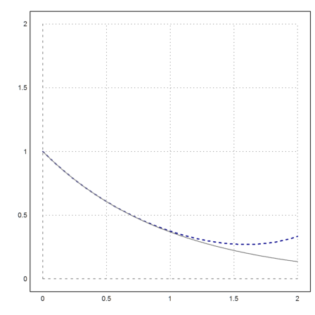
To fold all multi-lines press Ctrl+L. Then the subsequent lines will only be visible, if one of them has the focus. To fold a single multi-line start the first line with "%+ ".
>%+ x=4+5; ...
  // This line will not be visible once the cursor is off the line
A line starting with %% will be completely invisible.
81
Euler supports loops in command lines, as long as they fit into one single line or a multi-line. In programs, this restrictions does not hold, of course. For more information consult the following introduction.
>x=1; for i=1 to 5; x := (x+2/x)/2, end;
1.5
1.41666666667
1.41421568627
1.41421356237
1.41421356237
It is okay to use a multi-line. Make sure the line ends with " ...".
>x := 1.5; // comments go here before the ...
 repeat xnew:=(x+2/x)/2; until xnew~=x; ...
    x := xnew; ...
 end; ...
 x,
1.41421356237
Conditional structures do also work.
>if E^pi>pi^E; then "Thought so!", endif;
Thought so!
The primary data type in Euler is the real number. Reals are represented in IEEE format with about 16 decimal digits of accuracy.
>longest 1/3
0.3333333333333333
The internal dual representation takes 8 bytes.
>printdual(1/3)
1.0101010101010101010101010101010101010101010101010101*2^-2
>printhex(1/3)
5.5555555555554*16^-1
The default output format of EMT prints 12 digits. To make sure that we see the default, we reset the format.
>defformat; pi
3.14159265359
Internally, EMT uses the IEEE standard for double numbers with about 16 decimal digits. To see the full number of digits, use the command "longestformat", or we use the operator "longest" to display the result in the longest format.
>longest pi
3.141592653589793
Here is the internal hexadecimal representation of a double number.
>printhex(pi)
3.243F6A8885A30*16^0
The output format can be changed permanently with a format command.
>format(12,5); 1/3, pi, sin(1)
    0.33333
    3.14159
    0.84147
The default is format(12).
>format(12); 1/3
0.333333333333
Functions like "shortestformat", "shortformat", "longformat" work for vectors in the following way.
>shortestformat; random(3,8)
  0.66    0.2   0.89   0.28   0.53   0.31   0.44    0.3
  0.28   0.88   0.27    0.7   0.22   0.45   0.31   0.91
  0.19   0.46  0.095    0.6   0.43   0.73   0.47   0.32
The default format for scalars is format(12). But this can be changed.
>setscalarformat(5); pi
3.1416
The function "longestformat" set the scalar format too.
>longestformat; pi
3.141592653589793
For reference, here is a list of the most important output formats.
 shortestformat shortformat longformat, longestformat
 format(length,digits) goodformat(length)
 fracformat(length)
 defformat
The format can also be changed for the next print with the following operators.
shortest short long longest fraction
>longest pi, shortest pi
      3.141592653589793
   3.1
To reset the format, use defformat() or reset().
>defformat;
The print() function can be used to format a number in specific ways. It can add a unit, separate groups of digits with a hard space and use a decimal comma.
>print(1234567.789,2,20," "+euro$,true,",")
1 234 567,79 €
It is easy to define an operator for such prints.
>function prefix dollar (x) := print(x,2,unit=" $",>sep);
>dollar 1234.678
1 234.68 $
You can also set your own fancy format as a default format.
>function myformat(x) := print(x,2,15,>sep); ...
 userformat("myformat");
Then this format will be applied to every output.
>random(3,3)*100000
      52 518.36       50 225.52       16 860.35
      26 225.32       86 658.66       53 613.72
      49 345.33       60 134.38       65 946.08
>reset;
There is a special function %userprint(), which you can overwrite and use with the operator "uprint".
>function overwrite %userprint(x) := print(x,0,5,>sep); ...
 uprint 12312321.234234
12 312 321
Variables can be printed with their name using the operator "show".
>M=random(2,2); show M
M =
     0.967468      0.193151
     0.935921     0.0728753
Note that large Matrices are eclipsed by default.
>random(2,10)
Real 2 x 10 matrix

     0.988966     0.0104376      0.356626       0.52143     ...
     0.324407      0.340388      0.195494       0.44607     ...
To see the full matrix either switch off the default behavior or use "showlarge".
>largematrices on; random(2,10), largematrices off;
Column 1 to 5:
     0.469159      0.898763      0.388543      0.674114     0.0752676
      0.60809       0.10999      0.615836      0.217391      0.962872
Column 6 to 10:
     0.854693      0.123222      0.205006      0.465049     0.0281269
     0.842267      0.328758      0.561146      0.918802      0.997492
>showlarge random(2,10)
Column 1 to 5:
     0.473212      0.185709      0.421585      0.720843      0.247804
     0.224336     0.0102885      0.164816      0.356866      0.408866
Column 6 to 10:
     0.834083       0.44372      0.371866      0.775718       0.37468
     0.350091      0.347412      0.161257      0.588325       0.83884
The function printstr() can be used to print a string to a given length, left or right justified or centered, with a given fill character.
>printstr("Test",10,0,"-")
---Test---
>s=""; for i=1:5; s=s+"|"+printstr("Test",10,0); end; s+"|",
| Test | Test | Test | Test | Test |
>printstr(""+24,10,1,"0")
0000000024
Euler can convert units, but it does not check if the conversion makes sense. The units are stored in global variables, which end with "$". These variables are globally visible in functions.
>rEarth$, cm$,
6356752
0.01
A unit variable can be appended to a number to convert from the unit to the standard units (IS system). If a unit is used like this, the "$" can be omitted.
>5inch
0.127
There is a special operator -> to convert units, which converts either to a number or to a string.
>5km/hour->miles/day, 5kJ->" cal"
74.5645430685
5000 cal
It is safest to use units with the dollar sign because variables with the same name override the unit. In the following example, the value of the variable kts is not used for the unit kts$ (knots = nm/hour).
>kts=0; 190kts$ -> " km/h"
0.391240602667 km/h
Here is a list of all units in Euler. It includes some other variables, which are defined with $.
The units module does also contain some functions.
>FahrenheitToCelsius(100)
37.7777777778
There is also a very general print command, which can print a number with units.
>print(FahrenheitToCelsius(100),2,unit="°F")
37.78°F
It is easy to define own units.
>impgallon$=4.54609liter, 2.5impgallon->" l"
0.00454609
11.365225 l
For more details, see the introduction on complex numbers.
Complex numbers are entered using the constant I or with the 1i syntax.
>I^2, 1+3i
-1+0i
1+3i
Euler uses the principal values to compute logarithms and square roots for complex numbers, making these functions analytic in the plane cut along the negative axis.
>sqrt(-1+0.01i), sqrt(-1-0.01i),
0.00499994+1.00001i
0.00499994-1.00001i
Some functions return complex values by default. The values can be made real, if they are real. If they are not within the numerical accuracy epsilon(), an error will be generated.
An example is the function polysolve(), which finds the roots of a polynomial. We apply it to the Chebyshev polynomial of degree 5.
>real(polysolve(chebpoly(5)))
[0, 0.587785, 0.951057, -0.587785, -0.951057]
For details about intervals, see the following introduction.
Intervals are entered using the plus/minus character (F8), or the with the ~a,b~ notation.
>1±0.1, ~0.7,1.3~
~0.9,1.1~
~0.7,1.3~
The basic rule for intervals is:
Operators and functions compute all possible results for all numbers in each parameter interval, and find an enclosing interval for all these results.
The resulting interval is not always the smallest possible. But for the usual operators, it is very close to the optimal interval.
>~0,2~*~3,4~, ~-1,1~^2, cos(~1,5~)
~0,8~
~0,1~
~-1,0.54~
There are functions for guaranteed inclusions of solutions in Euler. These functions return intervals or vectors of intervals. An example is ilgs(), which returns an inclusion for the solution of linear systems.
>ilgs(hilbert(8),sum(hilbert(8)))
~0.999999999999999778,1.00000000000000022~
~0.999999999999999778,1.00000000000000022~
~0.999999999999999667,1.00000000000000022~
 ~0.999999999999998002,1.000000000000002~
~0.999999999999998668,1.00000000000000111~
~0.99999999999999778,1.00000000000000244~
~0.999999999999997891,1.00000000000000178~
~0.999999999999999556,1.00000000000000067~
The following tutorials contain more details about vectors, matrices, and the matrix language of Euler.
01 - The Matrix Language
04 - Linear Algebra
A matrix is entered using "[...]" with the values in each row separated by commas, the rows separated by semicolons. You may wish to select a shorter format for output.
>shortest [1,2,3;4,5,6]
     1      2      3
     4      5      6
By default, row vectors are printed in a compact format.
>[1,2,3,4]
[1, 2, 3, 4]
For matrices the special operator . denotes matrix multiplication, and A' denotes transposing. A 1x1 matrix can be used just like a real number.
>v:=[1,2]; v.v', %^2
5
25
Operators and functions obey the matrix language of Euler. For details, see the tutorial about the matrix language.
Here is just a summary of the rules.
E.g., a scalar value times a vector multiplies the value with each element of the vector. Or a matrix times a vector (with *, not .) expands the vector to the size of the matrix by duplicating it.
The following is a simple case with the operator ^.
>[1,2,3]^2
[1, 4, 9]
Here is a more complicated case. A row vector times a column vector expands both by duplicating.
>v:=[1,2,3]; v*v'
            1             2             3
            2             4             6
            3             6             9
Note that the scalar product uses the matrix product, not the *!
>v.v'
14
There are numerous functions for matrices. We give a short list. You should to consult the documentation for more information on these commands.
sum,prod computes the sum and products of the rows
cumsum,cumprod does the same cumulatively
min,max computes the extremal values of each row
extrema returns a vector with the extremal information
diag(A,i) returns the i-th diagonal
setdiag(A,i,v) sets the i-th diagonal
id(n) the identity matrix
det(A) the determinant
charpoly(A) the characteristic polynomial
eigenvalues(A) the eigenvalues
>v*v, sum(v*v), cumsum(v*v)
[1,  4,  9]
14
[1,  5,  14]
The : operator generates an equally spaces row vector, optionally with a step size.
>1:4, 1:2:10
[1,  2,  3,  4]
[1,  3,  5,  7,  9]
To concatenate matrices and vectors there are the operators "|" and "_".
>[1,2,3]|[4,5], [1,2,3]_1
[1,  2,  3,  4,  5]
            1             2             3
            1             1             1
The elements of a matrix are referred with "A[i,j]".
>A:=[1,2,3;4,5,6;7,8,9]; A[2,3]
6
For row or column vectors, v[i] is the i-th element of the vector. For matrices, this returns the complete i-th row of the matrix.
>v:=[2,4,6,8]; v[3], A[3]
6
[7,  8,  9]
The indices can also be row vectors of indices. : denotes all indices.
>v[1:2], A[:,2]
[2,  4]
            2
            5
            8
A short form for : is omitting the index completely.
>A[,2:3]
            2             3
            5             6
            8             9
For purposes of vectorization, the elements of a matrix can be accessed as if they were vectors.
>A{4}
4
A matrix can also be flattened, using the redim() function. This is implemented in the function flatten().
>redim(A,1,prod(size(A))), flatten(A)
[1,  2,  3,  4,  5,  6,  7,  8,  9]
[1,  2,  3,  4,  5,  6,  7,  8,  9]
A string in Euler is defined with "...".
>"A string can contain anything."
A string can contain anything.
Strings can be concatenated with | or with +. This also works with numbers, which are converted to strings in that case.
>"The area of the circle with radius " + 2 + " cm is " + pi*4 + " cm^2."
The area of the circle with radius 2 cm is 12.5663706144 cm^2.
The print function does also convert a number to a string. It can take a number of digits and a number of places (0 for dense output), and optimally a unit.
>"Golden Ratio : " + print((1+sqrt(5))/2,5,0)
Golden Ratio : 1.61803
There is a special string none, which does not print. It is returned by some functions, when the result does not matter. (It is returned automatically, if the function does not have a return statement.)
>none
To convert a string to a number simply evaluate it. This works for expressions too (see below).
>"1234.5"()
1234.5
To define a string vector, use the vector [...] notation.
>v:=["affe","charlie","bravo"]
affe
charlie
bravo
The empty string vector is denoted by [none]. String vectors can be concatenated.
>w:=[none]; w|v|v
affe
charlie
bravo
affe
charlie
bravo
Strings can contain Unicode characters. Internally, these strings contain UTF-8 code. To generate such a string, use u"..." and one of the HTML entities as described in
Unicode strings can be concatenated like other strings.
>u"α = " + 45 + u"°"
α = 45°
In plots, the strings will use the correct characters of the font, if they are available in the current font.
>plot2d(["x^3-x","3*x^2"],style=["-","--"], ...
   title=u"φ : x → x³ - x", ...
   xl="x",yl=u"φ(x)",>vertical); ...
 labelbox([u"φ(x)",u"φ'(x)"], ...
   styles=["-","--"],x=0.1,>left):
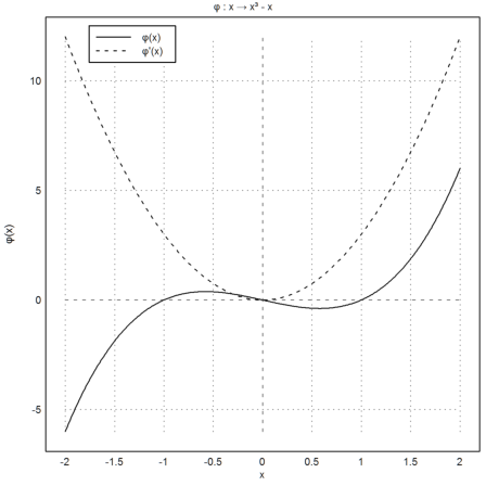
In comments, the same entities like α, β etc. can be used. This may be a quick alternative to Latex. (More details on comments below).
There are some functions to create or analyze unicode strings. The function strtochar() will recognize Unicode strings, and translate them correctly.
>v=strtochar(u"Ä is a German letter")
[196,  32,  105,  115,  32,  97,  32,  71,  101,  114,  109,  97,  110,
32,  108,  101,  116,  116,  101,  114]
The result is a vector of Unicode numbers. The converse function is chartoutf().
>v[1]=strtochar(u"Ü")[1]; chartoutf(v)
Ü is a German letter
The function utf() can translate a string with entities in a variable into a Unicode string.
>s="We have α=β."; utf(s)
We have α=β.
It is also possible to use numerical entities.
>u"Ähnliches"
Ähnliches
Boolean values are represented with 1=true or 0=false in Euler. Strings can be compared, just like numbers.
>2<1, "ape"<"banana"
0
1
"and" is the operator "&&" and "or" is the operator "||", as in the C language. (The words "and" and "or" can only be used in conditions for "if".)
>2<E && E<3
1
Boolean operators obey the rules of the matrix language.
>(1:10)>5, nonzeros(%)
[0,  0,  0,  0,  0,  1,  1,  1,  1,  1]
[6,  7,  8,  9,  10]
You can use the function nonzeros() to extract specific elements form a vector. In the example, we use the conditional isprime(n).
>N=2|3:2:99; N[nonzeros(isprime(N))]
[2,  3,  5,  7,  11,  13,  17,  19,  23,  29,  31,  37,  41,  43,  47,
53,  59,  61,  67,  71,  73,  79,  83,  89,  97]
For examples of numerical expressions, have a look at the following first introduction.
Strings can contain mathematical expressions, which can be evaluated by EMT. For this, use parentheses after the expression. If you intend to use a string as an expression, use the convention to name it "fx" or "fxy" etc. Expressions take precedence over functions.
Global variables can be used in the evaluation.
>r:=2; fx:="pi*r^2"; longest fx()
12.56637061435917
Parameters are assigned to x, y, and z in that order. Additional parameters can be added using assigned parameters.
>fx:="a*sin(x)^2"; fx(5,a=-1)
-0.919535764538
Note that expression will always use global variables, even if there is a variable in a function with the same name. (Otherwise the evaluation of expressions in functions could have very confusing results for the user that called the function.)
>at:=4; function f(expr,x,at) := expr(x); ...
 f("at*x^2",3,5) // computes 4*3^2 not 5*3^2
36
If you want to use another value for "at" than the global value you need to add "at=value".
>at:=4; function f(expr,x,a) := expr(x,at=a); ...
 f("at*x^2",3,5)
45
For reference, we remark that call collections (discussed elsewhere) can contain expressions. So we can make the above example as follows.
>at:=4; function f(expr,x) := expr(x); ...
 f({{"at*x^2",at=5}},3)
45
Expressions in x are often used just like functions. E.g., the following command plots a function in x and y.
>plot3d("x*y^2",r=2,angle=-48°,zoom=2.2):
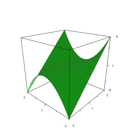
Note that defining a function with the same name like a global symbolic expression deletes this variable to avoid confusion between symbolic expressions and functions.
>f &= 5*x;
>function f(x) := 6*x;
>f(2)
12
By way of convention, symbolic or numerical expressions should be named fx, fxy etc. This naming scheme should not be used for functions.
>fx &= diff(x^x,x)
                            x
                           x  (log(x) + 1)
A special form of an expression allows any variable as an unnamed parameter to the evaluation of the expression, not just "x", "y" etc. For this, start the expression with "@(variables) ...".
>"@(a,b) a^2+b^2", %(4,5)
@(a,b) a^2+b^2
41
This allows to manipulate expressions in other variables for functions of EMT which need an expression in "x".
>"a^2+a+1"; plot2d("@(a) "+%):
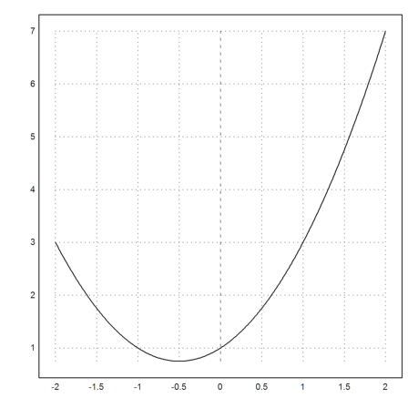
Symbolic expressions and variables are explained in detail in the following introduction.
Symbolic expressions are special strings in Euler. They are defined with "&...". Euler scans the input to find the end of the symbolic expression automatically.
Symbolic expressions are printed by Maxima in 2D form. The reason for this is a special symbolic flag in the string.
>&(3+x)/(x^2+1)
                                x + 3
                                ------
                                 2
                                x  + 1
Symbolic expressions are parsed by Euler. If you need a complex syntax in one expression, you can enclose the expression in "...". To use more than a simple expression is possible, but strongly discouraged.
>&"v := 5; v^2"
25
For completeness, we remark that symbolic expressions can be used in programs, but need to be enclosed in quotes. Moreover, it is much more effective to call Maxima at compile time if possible.
Symbolic variables are defined with "&=".
>fx &= (x+1)/(x^4+1)
                                x + 1
                                ------
                                 4
                                x  + 1
Symbolic expressions can be used in other symbolic expressions.
>&factor(diff(fx,x))
                               4      3
                          - 3 x  - 4 x  + 1
                          -----------------
                                4     2
                              (x  + 1)
If you have Latex installed, you can print a symbolic expression with Latex. If not, the following command will issue an error message.
Learn about how to install Latex for Euler in the documentation.
To print a symbolic expression with Latex, use $... instead of &... Do not run the following command, if you don't have Latex installed.
>$factor(diff(fx,x,2))
![]()
To get the Latex code for an expression, you can use the tex command.
>tex(fx)
\frac{x+1}{x^4+1}
Symbolic expressions can be evaluated just like numerical expressions.
>fx(0.5)
1.41176470588
In symbolic expressions, this does not work, since Maxima does not support it. Instead, use the "with" syntax (a nicer form of the at(...) command of Maxima).
>&fx with x=1/2
                                  24
                                  --
                                  17
The assignment can also be symbolic.
>&fx with x=1+t
                                t + 2
                             ------------
                                    4
                             (t + 1)  + 1
Symbolic expressions can be plotted just like numerical expressions.
>plot2d(fx,-1,1); plot2d(&diff(fx,x),>add,color=red):
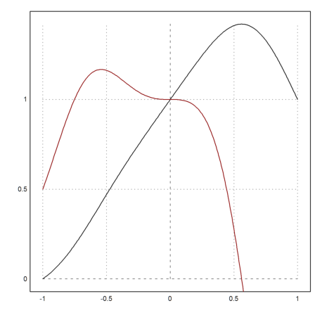
The command solve solves symbolic expressions for a variable in Maxima. The result is a vector of solutions.
>&solve(x^2+x=4,x)
                     - sqrt(17) - 1      sqrt(17) - 1
                [x = --------------, x = ------------]
                           2                  2
Compare with the numerical "solve" command in Euler, which needs a start value, and optionally a target value.
>solve("x^2+x",1,y=4)
1.56155281281
The numerical values of the symbolic solution can be computed by evaluation of the symbolic result. Euler will read over the assignments x= etc. If you do not need the numerical results for further computations you can also let Maxima find the numerical values.
>sol &= solve(x^2+2*x=4,x), sol(), &float(sol)
                 [x = - sqrt(5) - 1, x = sqrt(5) - 1]

[-3.23607,  1.23607]

            [x = - 3.23606797749979, x = 1.23606797749979]
To get a specific symbolic solution, one can use "with" and an index.
>&solve(x^2+x=1,x), x2 &= x with %[2]
                      - sqrt(5) - 1      sqrt(5) - 1
                 [x = -------------, x = -----------]
                            2                 2


                             sqrt(5) - 1
                             -----------
                                  2
To solve a system of equations, use a vector of equations. The result is a vector of solutions.
>sol &= solve([x+y=3,x^2+y^2=5],[x,y]), &x*y with sol[1]
                   [[x = 2, y = 1], [x = 1, y = 2]]


                                  2
Symbolic expressions can have flags, which indicate a special treatment in Maxima. Some flags can be used as commands too, others can't. Flags are appended with "|" (a nicer form of "ev(...,flags)")
>& diff((x^3-1)/(x+1),x) | ratsimp
                              3      2
                           2 x  + 3 x  + 1
                           ---------------
                             2
                            x  + 2 x + 1
EMT can handle lists in two ways. First there are global lists, which are useful to put global elements in one place to be accessed everywhere.
The following is a list of 1000 vectors.
>glist("test"); for i=1 to 1000; glistadd("test",1:i); end;
>glistget("test",10), glistget("test",11)
[1,  2,  3,  4,  5,  6,  7,  8,  9,  10]
[1,  2,  3,  4,  5,  6,  7,  8,  9,  10,  11]
To get rid of a list, remove it.
>glistremove("test");
There are also collections, which behave like ordinary variables. In contrast to the global lists, they are immutable once they are constructed. Collections can contain any value of EMT.
>a={{"element"+1,2,3+I}}; a,
element1
2
3+1i
The elements are addressed by numbers.
>a[2]
2
A special type of collections is used in algorithms which need a numerical function or expression. The first element is the name of the function or the expression, and the later elements are additional arguments. We call that a "call collection".
>function f(x,a) := x^a
>integrate({{"f",4}},0,1)
0.2
This works also with expressions. But the extra parameters must be named then. (Usually, naming an element of a collection has no effect.)
For an example, we call the numerical integrator of EMT for x^4.
>integrate({{"x^a",a=4}},0,1)
0.2
Some functions return more then one value. E.g., the function sort() returns the sorted vector and the rearrangement of indices. Multiple return values of a function can be placed in a collection in the following way.
>x=random(10); L={{sort(x)}}
[0.058542,  0.0960726,  0.132256,  0.164719,  0.236419,  0.385195,
0.448604,  0.906718,  0.916402,  0.945399]
[10,  3,  9,  5,  6,  4,  8,  1,  2,  7]
In this overview, we cover only one-line functions. For more complex functions, see the introduction to programming.
A numerical one-line function is defined by ":=".
>function f(x) := x*sqrt(x^2+1)
For an overview, we show all possible definitions for one-line functions. The details will be covered later.
function f(x) := exp(x) // numerical function
function f(x) &= diff(x*exp(x),x) // symbolic function
function D(f,x) &&= D(f,x)+D(f,x,2) // purely symbolic function
A function can be evaluated just like any built-in Euler function.
>f(2)
4.472135955
This function will work for vectors too, obeying the matrix language of Euler, since the expressions used in the function are vectorized.
>f(0:0.1:1)
[0,  0.100499,  0.203961,  0.313209,  0.430813,  0.559017,  0.699714,
0.854459,  1.0245,  1.21083,  1.41421]
Functions can be plotted. Instead of expressions, we need only provide the function name.
In contrast to symbolic or numerical expressions, the function name must be provided in a string.
>plot2d("f",-1,1):
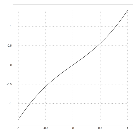
plot2d, plot3d and other commands understand strings, containing the function name.
>solve("f",1,y=1)
0.786151377757
By default, if you need to overwrite a built-in function, you must add the keyword "overwrite". Overwriting built-in functions is dangerous and can cause problems for other functions depending on them.
You can still call the built-in function as "_...", if it is function in the Euler core.
>function overwrite sin (x) := _sin(x°) // computes sine in degrees
>sin(45)
0.707106781187
We better remove this redefinition of sin.
>forget sin; sin(pi/4)
0.707106781187
Numerical function can have default parameters.
>function f(x,a=1) := a*x^2
Omitting this parameter uses the default value.
>f(4)
16
Setting it overwrites the default value.
>f(4,5)
80
An assigned parameter overwrite it too. This is used by many Euler functions like plot2d, plot3d.
>f(4,a=1)
16
If a variable is not a parameter, it must be global. One-line functions can see global variables.
>function f(x) := a*x^2
>a=6; f(2)
24
But an assigned parameter overrides the global value.
If the argument is not in the list of pre-defined parameters, it must be declared with ":="!
>f(2,a:=5)
20
There is a special form to assign the value false=0 and true=1 to an assigned parameter.
>flag : flag=true
<flag : flag=false
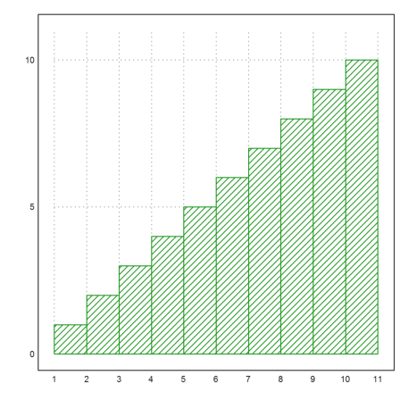
This makes the meaning of parameters more clear to the reader. In the example we want a bar plot.
>plot2d(1:10,>bar,style="/"):
Many details can be found in the introduction to Maxima in Euler.
Symbolic functions are defined with "&=". They are defined in Euler and Maxima, and work in both worlds. The defining expression is run through Maxima before the definition.
>function g(x) &= x^3-x*exp(-x)
                              3      - x
                             x  - x E
Symbolic functions can be used in symbolic expressions.
>&diff(g(x),x), &% with x=4/3
                            - x    - x      2
                         x E    - E    + 3 x


                              - 4/3
                             E        16
                             ------ + --
                               3      3
They can also be used in numerical expressions. Of course, this will only work if EMT can interpret everything inside the function.
>g(5+g(1))
178.635099908
They can be used to define other symbolic functions or expressions.
>function G(x) &= factor(integrate(g(x),x))
                         - x   4  x
                        E    (x  E  + 4 x + 4)
                        ----------------------
                                  4
They can be plotted, since they are also numerical functions.
>plot2d("g",-1,1):
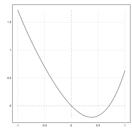
They can also be plotted or used in symbolic form if they appear in a symbolic expression.
>solve(&g(x),0.5)
0.703467422498
The following works too, since Euler uses the symbolic expression in the function g, if it does not find a symbolic variable g, and if there is a symbolic function g.
>solve(g,0.5)
0.703467422498
Euler allows underscores in names. But they need to be doubled.
>function gamma__incomplete__regularized(a,b) := gammaic(b,a)
>gamma__incomplete__regularized(3,4)
0.238103305554
Maxima has the same function gamma_incomplete_regularized, but would not understand the double underscore. So this is translated on the way between Euler and Maxima.
Assume, we define an expression.
>fx &= gamma_incomplete__regularized(x,y)
gamma_incomplete_regularized(x, y)
In EMT, this is stored with a double underscore.
>""|fx
gamma__incomplete__regularized(x,y)
Thus it can be evaluated by EMT numerically. Note that we defined the function "gamma__incomplete__regularized" numerically above. Also, note that the following effectively uses the function gammaic() from EMT.
>fx(3,4)
0.238103305554
In Maxima it is stored with a single underscore. Thus it can be evaluated in Maxima. Note that the following is using the "gamma_incomplete_regularized" function from Maxima.
>&float(fx with [x=3,y=4])
0.2381033055535436
The usual [...] form to define matrices can be used in Euler to define symbolic matrices.
>A &= [1,a;b,2]
                               [ 1  a ]
                               [      ]
                               [ b  2 ]
Like all symbolic variables, these matrices can be used in other symbolic expressions.
>&det(A-x*ident(2)), &solve(%,x)
                        (1 - x) (2 - x) - a b


               3 - sqrt(4 a b + 1)      sqrt(4 a b + 1) + 3
          [x = -------------------, x = -------------------]
                        2                        2
The eigenvalues can also be computed automatically. The result is a vector with two vectors of eigenvalues and multiplicities.
>&eigenvalues([a,1;1,a])
[[a - 1, a + 1], [1, 1]]
To extract a specific eigenvector needs careful indexing.
>&eigenvectors([a,1;1,a]), &%[2][1][1]
          [[[a - 1, a + 1], [1, 1]], [[[1, - 1]], [[1, 1]]]]


                               [1, - 1]
Symbolic matrices can be evaluated in Euler numerically just like other symbolic expressions.
>A(a=4,b=5)
            1             4
            5             2
In symbolic expressions, use with.
>&A with [a=4,b=5]
                               [ 1  4 ]
                               [      ]
                               [ 5  2 ]
Access to rows of symbolic matrices work just like with numerical matrices.
>&A[1]
[1, a]
A symbolic expression can contain an assignment. And that changes the matrix A.
>&A[1,1]:=t+1; &A
                             [ t + 1  a ]
                             [          ]
                             [   b    2 ]
There are symbolic functions in Maxima to create vectors and matrices. For this, refer to the documentation of Maxima or to the tutorial about Maxima in EMT.
>v &= makelist(1/(i+j),i,1,3)
                           1      1      1
                        [-----, -----, -----]
                         j + 1  j + 2  j + 3
A symbolic expression is just a string containing an expression. If we want to define a value both for symbolic expressions and for numerical expressions, we must use "&:=".
>A &:= [1,pi;4,5]
            1       3.14159
            4             5
There is still a difference between the numerical and the symbolic form. When transferring the matrix to the symbolic form, fractional approximations for reals will be used.
>&A
                            [    1146408 ]
                            [ 1  ------- ]
                            [    364913  ]
                            [            ]
                            [ 4     5    ]
To avoid this, there is the function "mxmset(variable)".
>mxmset(A); &A
                       [ 1  3.141592653589793 ]
                       [                      ]
                       [ 4          5         ]
Maxima can also compute with floating point numbers, and even with big floating numbers with 32 digits. The evaluation is much slower, however.
>&bfloat(sqrt(2)), &float(sqrt(2))
                 1.4142135623730950488016887242097b0


                          1.414213562373095
The precision of the big floating point numbers can be changed.
>&fpprec:=100; &bfloat(pi)
        3.14159265358979323846264338327950288419716939937510582097494\
4592307816406286208998628034825342117068b0
A numerical variable can be used in any symbolic expressions using "@var".
Note that this is only necessary, if the variable has been defined with ":=" or "=" as a numerical variable.
>B:=[1,pi;3,4]; &det(@B)
- 5.424777960769379
Symbolic functions can be defined for symbolic use only. Use "&&=" in the function definition.
This is necessary, if the function can not work numerically, or does purely symbolic stuff only.
>function D(f,x) &&= diff(f,x)+x*diff(f,x,2)
diff(f, x, 2) x + diff(f, x)
Symbolic functions are not evaluated when they are defined. They work like macros in Maxima.
>&D(exp(x^2),x)
                              2       2          2
                          2  x       x          x
                    x (4 x  E   + 2 E  ) + 2 x E
For examples to the topic of this sections, see the introduction to programming.
Many functions, like plot2d, accept functions and expressions as parameters.
In case of expressions, the variables x or y are used e.g. by plot3d. Other variables must be global. In case of functions, plot3d passes the variables x and y to the function. Other variables must be passed by semicolon parameters.
Have a look into the documentation about programming how this is handled inside the function plot3d.
>function f(x,a) := a*x^2
>plot2d("f",-1,1;0.5); // with a=0.5 ...
 insimg;
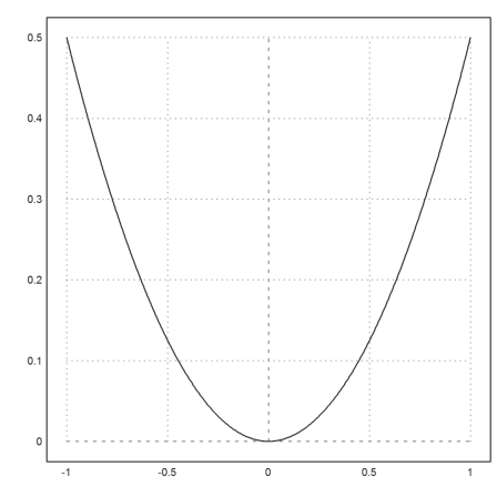
Note that by internal reasons assigned parameters cannot be defined before the semicolon parameters. Assigned parameters must be added as last parameters, as in the following example.
>plot2d("f";0.5,r=2):
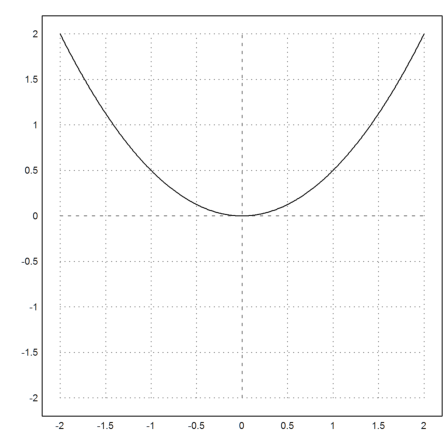
Call collections are another way to achieve the same. Instead of the function name, the parameter is a call collection with the function name and additional parameters.
>plot2d({{"f",0.5}},0,2,thickness=2):
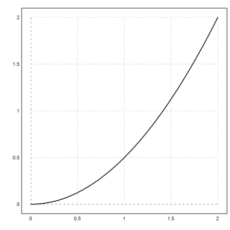
In case of expression, the additional parameters must be named.
>plot3d({{"a*x^2+a^2*x*y+y^2",a=2}},>spectral):
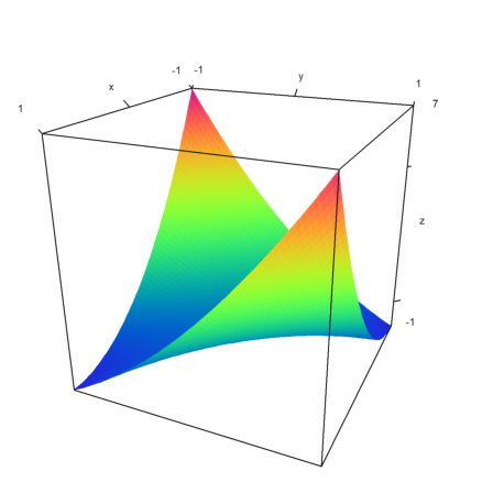
Some functions do not work for vector input. Here is an example.
We wish to define the inverse of the following function numerically.
>function f(t) := t*sqrt(t^2+1)
The function s=f(x) is monotone and has an inverse function for positive values of s.
>plot2d("f",0,5,xl="x",yl="s=f(x)",grid=7):
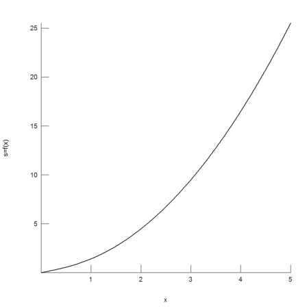
We define the inverse function by solving f(x)=s for x. We use the numerical solve algorithm of Euler with a starting value s, and target value y=s.
>function map invf(s) := solve("f(x)",s,y=s)
It does indeed work.
>invf(f(2))
2
The map keyword in the definition of the function makes it work for vectors too. The function is simply applied to all elements of the parameter, if it is a vector.
>f(invf(1:5))
[1, 2, 3, 4, 5]
For another example, we define the function
![]()
>function map F(t) := integrate("f",0,t);
>plot2d("F",0,2,xl="t",yl="F(t)"):
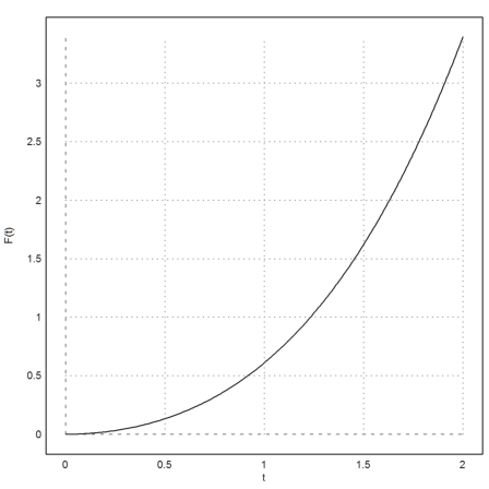
The comment editor of Euler knows lines of text, which it wraps into paragraphs. For the reader, it is convenient to have one line of space between normal paragraphs. Comments should be formatted with a fixed font, in Euler and in the HTML output. The default width is 80 characters.
Euler comments can contain headings, Latex equations, links and images. All these items are lines starting with a special sequence of characters. The heading above has been generated with
* Syntax of Euler Comments
with the * at the first place of the line.
As you see, an empty line with an empty command is hidden.
A subheading can be generated with
** Subheadings
You can also get a vertical line only with
---
Other items in a line are formulas. Here examples of the two possible forms
 latex: \int_0^1 x^2 \, dx = \frac{1}{3}
 maxima: 'integrate(x^2,x,0,1) = integrate(x^2,x,0,1)
The result is
![]()
![]()
The second result was computed by Maxima, with 'integrate on the left side to prevent evaluation.
Of course, Latex must be installed properly for this, and the latex directory must be in the path. Or you can set the necessary binaries in the Options menu.
You can use AMS environments instead of display formulas in Latex. Use "latex: \begin{..." for this. The following is an example of align*.
latex: \begin{align*} a &= b+c \\ d &= e+f+g \end{align*}
![]()
Do not use numbered environments, since the number will always be 1.
You can also use your own definitions in a package. Put the file "eupng.sty" into the directory of the notebook.
Moreover, comments can contain links. The following are possible:
 http://euler.rene-grothmann.de
 See: 00 - The Syntax of Euler
 See: ../reference/eulercore.html#Units | Units
The result is
http://euler.rene-grothmann.de
00 - The Syntax of Euler
Units
These links will be properly exported to HTML. For the second link, the HTML file must be in the current directory, of course. This is the case for this introduction.
Another type of special lines are images. The syntax is
image: ../images/autor.jpg
The result is

This image is installed with Euler. You can also load an image into a command line of Euler.
>loadimg("../images/Icon.png");

It is possible to use MathJax for HTML export, or tp use SVG for all images. For more information, see the following introduction.